6.2 Global identifiability of the DINA or DINO model
We first consider the DINA or DINO model. We give the identifiability condition first, and then discuss the impact of nonidentifiability.
Identifiability Conditions #1
When DINA or DINO model is used, the following conditions are sufficient and necessary for global model identification of both item and population proportion parameters (G. Xu, 2019).
- The Q-matrix has the following forms, where \(I_K\) is an identity matrix. \[ Q=\begin{pmatrix} I_K \\ Q' \end{pmatrix} \]
- Each attribute is measured by at least three items.
- Any two different columns of \(Q'\) are distinct.
Now let’s check how nonidentifiability affects DINA model analysis.
Based on the identifiability conditions above, the Q-matrix below is not identified.
Code
Q <- matrix(c(1, 0, 0, 1, 1, 1, 1, 1, 1, 1), ncol = 2, byrow = TRUE)| Attribute 1 | Attribute 2 | |
|---|---|---|
| Item 1 | 1 | 0 |
| Item 2 | 0 | 1 |
| Item 3 | 1 | 1 |
| Item 4 | 1 | 1 |
| Item 5 | 1 | 1 |
The data in DINA_idf.csv was simulated based on the following parameters:
Code
g <- c(0.05, 0.1, 0.15, 0.2, 0.25)
s <- c(0.05, 0.1, 0.15, 0.2, 0.25)
p <- c(0.25, 0.25, 0.25, 0.25)
Let us fit the DINA model to the data using the code below. Please change the randomseed used to generate initial item parameters and see how that will affect the estimates.
Code
library(GDINA)
df <- read.csv("data/DINA_idf.csv")
DINA.est <- GDINA(df, Q, model = "DINA", control = list(conv.crit = 1e-06,
    randomseed = 123), verbose = FALSE)
coef(DINA.est, "gs")
## guessing slip
## Item 1 0.045 0.037
## Item 2 0.083 0.079
## Item 3 0.163 0.162
## Item 4 0.196 0.221
## Item 5 0.251 0.234Code
coef(DINA.est, "lambda")## p(00) p(10) p(01) p(11)
## 0.24 0.25 0.26 0.25Click for Findings
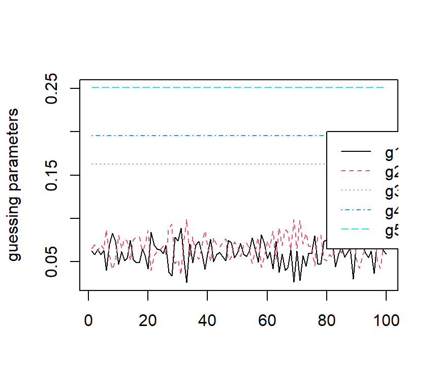
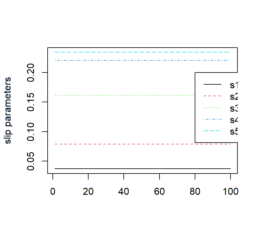
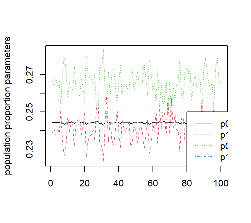
The figures below show the estimated DINA parameters as well as the negative two loglikelihood values with 100 sets different initial values. It can be observed that slip parameters seem to be identifiable, but guessing parameters for items 1 and 2, as well as the population proportion parameters for latent profile 00, 10 and 01 are not idnetifiable.


The code is given below:
Code
 library(GDINA)
 df <- read.csv("data/DINA_idf.csv")
 R <- 100
 output <- matrix(NA, R, 15)
 for (i in 1:R) {
     DINA.est <- GDINA(df, Q, model = "DINA", control = list(conv.crit = 1e-06,
         randomseed = i * 100), verbose = FALSE)
     output[i, ] <- c(coef(DINA.est, "gs"), coef(DINA.est, "lambda"), deviance(DINA.est))
 }
 output <- data.frame(output)
 colnames(output) <- c(paste0("g", 1:5), paste0("s", 1:5), "p00", "p10",
     "p01", "p11", "-2LL")


 matplot((output[, 1:5]), type = "l", ylab = "guessing parameters")
 legend(80, 0.2, legend = colnames(output)[1:5], col = 1:5, lty = 1:5)

 matplot((output[, 6:10]), type = "l", ylab = "slip parameters")
 legend(80, 0.2, legend = colnames(output)[6:10], col = 1:5, lty = 1:5)

 matplot((output[, 11:14]), type = "l", ylab = "population proportion parameters")
 legend(80, 0.25, legend = colnames(output)[11:14], col = 1:5, lty = 1:5)


 matplot(round(output[, 15], 4), type = "l", ylab = "-2 log likelihood")