6.4 Generic Identifiability for more general CDMs

Sufficient and necessary global identifiability conditions are difficult to find for R-RUM, ACDM, LLM and G-DINA model. Researchers have considered a generic identifiability, which ensures that the model is identified for most parameters.

Identifiability Conditions #4

G. Xu (2019) points out that main-effect models and saturated models are generically identified when the Q-matrix takes the following form

\[ Q=\begin{pmatrix} Q_1 \\ Q_2\\ Q^{\star} \end{pmatrix} \] where \(Q_1\) and \(Q_2\) take the following forms (\(*\) can be either 0 or 1):

\[ Q_i=\begin{pmatrix} 1 & * &\ldots&*\\ * & 1 &\ldots&*\\ \vdots & \vdots &&\vdots\\ *&*&\ldots&1 \end{pmatrix} \] and in \(Q^{\star}\), each attribute is required by at least one item.

The above conditions imply that each attribute should be measured at least three time.

Now let’s check how nonidentifiability affects LLM analysis.

Based on the generic identifiability conditions above, the Q-matrix below is not identified.

Code

Q <- matrix(c(1, 0, 0, 0, 1, 0, 0, 0, 1, 1, 0, 1, 1, 1, 0), ncol = 3, byrow = TRUE)

TABLE 6.2: Q-matrix

	Attribute 1	Attribute 2	Attribute 3
Item 1	1	0	0
Item 2	0	1	0
Item 3	0	0	1
Item 4	1	0	1
Item 5	1	1	0

The data in ACDM_idf.csv was simulated based on the following parameters:

Code

delta <- list(item1 = c(0.2, 0.5), item2 = c(0.3, 0.6), item3 = c(0.1,
    0.4), item4 = c(0.2, 0.3, 0.4), item5 = c(0.2, 0.2, 0.5))
p <- rep(1/8, 8)

Let us fit the ACDM model to the data using the code below. Please change the randomseed used to generate initial item parameters and see how that will affect the estimates.

Code

library(GDINA)
df <- read.csv("data/ACDM_idf.csv")
ACDM.est <- GDINA(df, Q, model = "ACDM", control = list(conv.crit = 1e-06,
    randomseed = 123), verbose = FALSE)
coef(ACDM.est, "delta")

## $`Item 1`
##   d0   d1 
## 0.28 0.48 
## 
## $`Item 2`
##   d0   d1 
## 0.36 0.64 
## 
## $`Item 3`
##    d0    d1 
## 0.082 0.914 
## 
## $`Item 4`
##   d0   d1   d2 
## 0.35 0.38 0.26 
## 
## $`Item 5`
##   d0   d1   d2 
## 0.33 0.17 0.42

Code

coef(ACDM.est, "lambda")

## p(000) p(100) p(010) p(001) p(110) p(101) p(011) p(111) 
##  0.308  0.191  0.166  0.078  0.111  0.037  0.061  0.047

Click for Findings

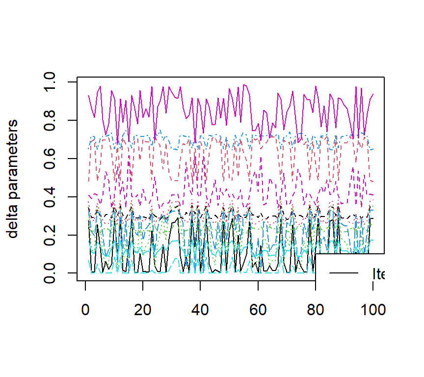
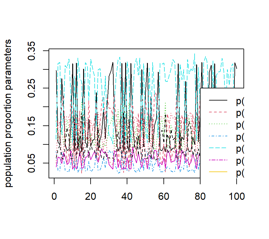
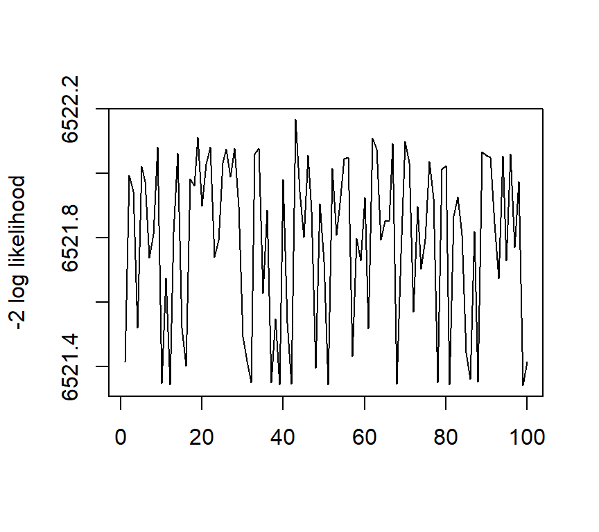
The figures below show the estimated ACDM parameters as well as the negative two loglikelihood values with 100 sets different initial values.

The code is given below:

Code

library(GDINA)
Q <- matrix(c(1, 0, 0, 0, 1, 0, 0, 0, 1, 1, 0, 1, 1, 1, 0), ncol = 3, byrow = TRUE)
df <- read.csv("data/ACDM_idf.csv")

R <- 100
output <- matrix(NA, R, 21)
for (i in 1:R) {
    ACDM.est <- GDINA(df, Q, model = "ACDM", control = list(conv.type = "neg2LL",
        conv.crit = 0.001, randomseed = 123 * i), verbose = FALSE)
    output[i, ] <- c(unlist(coef(ACDM.est, "delta")), coef(ACDM.est, "lambda"),
        deviance(ACDM.est))
}
output <- data.frame(output)
colnames(output) <- c(names(unlist(coef(ACDM.est, "delta"))), names(coef(ACDM.est,
    "lambda")), "-2LL")



matplot((output[, 1:12]), type = "l", ylab = "delta parameters")
legend(80, 0.1, legend = colnames(output)[1:12], col = 1:12, lty = 1:12)


matplot((output[, 13:20]), type = "l", ylab = "population proportion parameters")
legend(80, 0.25, legend = colnames(output)[13:20], col = 1:8, lty = 1:8)


matplot(round(output[, 21], 4), type = "l", ylab = "-2 log likelihood")

References

Xu, G. (2019). Identifiability and Cognitive Diagnosis Models (M. von Davier & Y.-S. Lee, Eds.; pp. 333–357). Springer International Publishing. http://link.springer.com/10.1007/978-3-030-05584-4_16